The Phi Accrual Failure Detector

Problem definition

Detecting failure in a distributed system setting is a desirable task for many obvious reasons. This paper introduces an implementation of an adaptive (accrual) failure detector. In this $\varphi$ accrual failure detector, the conditions of the network is accumulated and used to update the probabilistic model for failure suspicion. Compares to the existing models in 2004, which output of suspicion level is binary, this implementation has the advantage of returning a real-value suspicion level. The authors compared their implementation to Chen Fault Detection and Bertier Fault Detection. For the benchmark scheme, they set up two computers between Japan and Switzerland transferring “heart beat” signal from Japan. They then later analyzed the collected data over a week and reported the result.

Input: A set of master processes $\mathcal{M}$ and a set of worker processes $\mathcal{W}$ . The master processes are in charge of monitoring the worker processes.
Output: An indicator of failure for each worker processes.
Assumption: In this paper, for the shake of simplicity, the authors assumed that the master processes will never crash. Furthermore, only one worker and one master scheme was discussed in this paper.

Notations

Note: The setting in this paper is sending heart beat signals from Japan to Switzerland.

Notation	Explaination
$\varphi$	Suspection value. Higher value means the higher chance the failure happened.
$\Phi$	Hyperparameter. Threshold for $\varphi$ .
$\Delta_i$	”Heart beat” signal period.
$\Delta_{to}$	Timeout for transmission.
$\Delta_{tr}$	Average transmission time experienced by the messages.
$\alpha$	$\Delta_{tr} \approx \Delta_{i} + \alpha$
$q$	Master process that monitors other process for failure dection.
$p$	Worker process that sends “heart beat” signals.
$T_D$	Time until q begins to suspect p permanently in case of failure happened.
$\lambda_M$	Average mistake rate at which a failure detector generates wrong suspicions.
$\lozenge P$	Eventually perfect failure detector class.
$\mathrm{susp\_level\_p}(t)$	Suspicion level of p at time t.
$T_{high}$	Dynamic threshold upperbounds $susp\_level_p$ .
$T_{low}$	Dynamic threshold lowerbounds $susp\_level_p$ .
$T_{last}$	The time when thest most recent heart beat was received.
$t_{now}$	The current time.
$P_{later}(t)$	The probability that the next heart beat will arrive after $t$ time unit since the last one.

Method

As mentioned above, this paper proposed an abstract accrual failure detector and a simple implementation of the idea with only 2 processes. This figure illustrates the differences in the conventional failure detection architecture and the proposed accrual failure detection architecture.

phifail

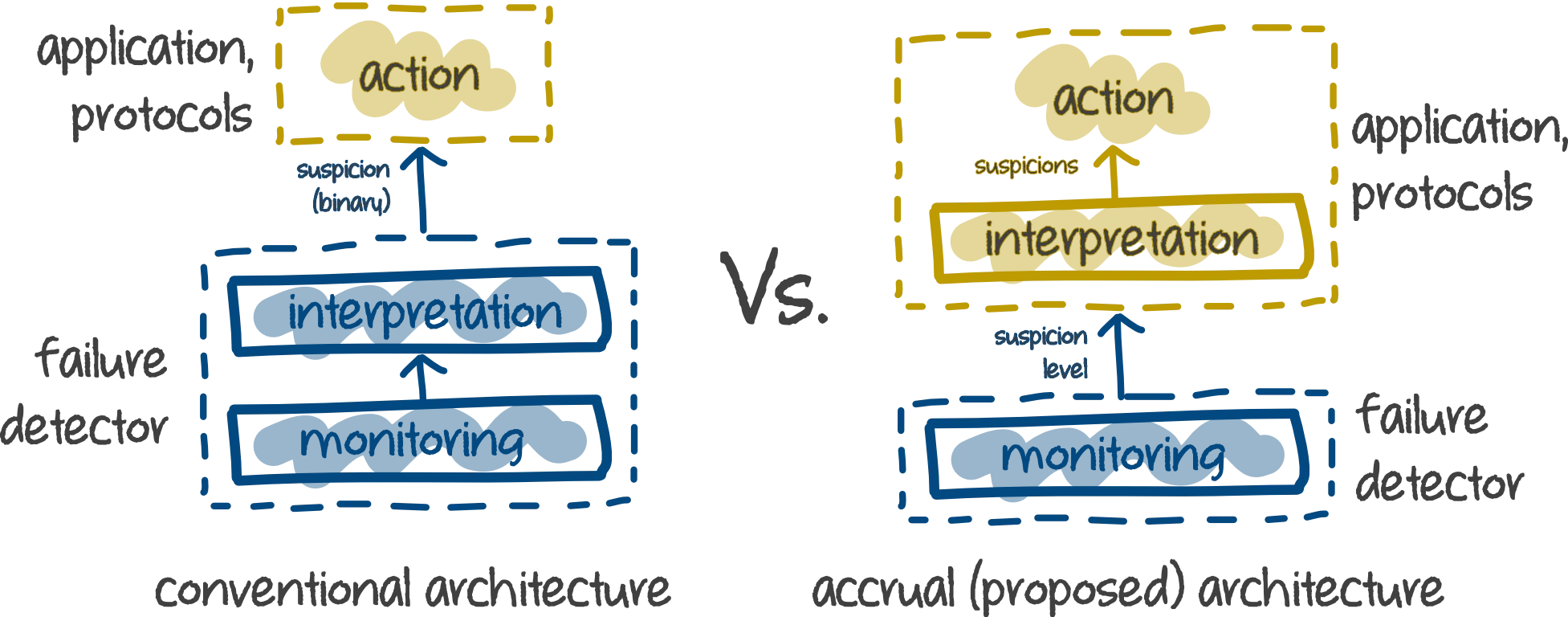
The main different in the proproposed architecture is the ability to return many suspicion levels instead of just binary levels. This scheme enable the system to perform many action as well as adaptive action based on the suspicion input level. In the proposed architecture, the suspicion level is represented by a value called $\varphi$ . The suspicion level is defined by a logarithmic scale:

$\varphi(t_{now}) \triangleq -\log_{10}(P_{later}(t_{now} - T_{last}))$

This formula is intuitive in the sense that it penaltize the delay $t_{now} - T_{last}$ by a log scale of some pre-defined probabilistic model $P_{later}(t)$ . In this paper, the authors defined a threshold $\Phi$ for $\varphi$ . Since this $\varphi$ variable is computed in the log-scale, $\Phi$ also has logarithmic meaning. Each of the unit step increase of $\Phi$ will lead to ten times confident interval of failure detection. However, this fact only means that the confident about a failure dection is high, it doesn’t take into account the speed of the dectection.

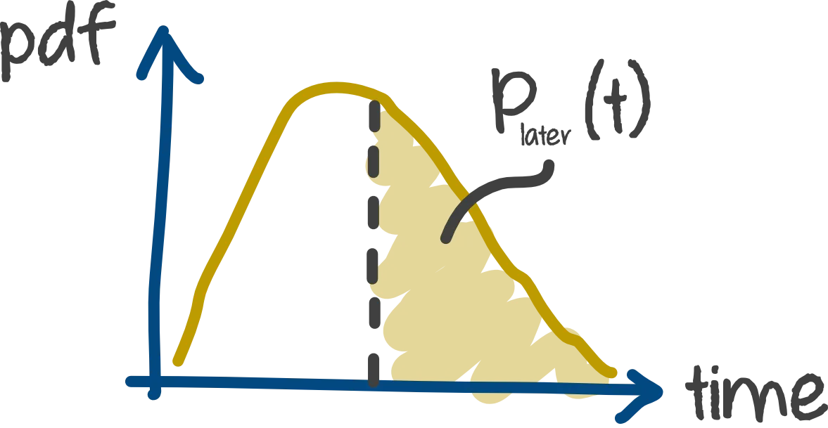
The probabilistic model is given by the formula:

\begin{align} P_{later}(t) &= \frac{1}{\sigma \sqrt{2\pi}} \int_{t}^{+\infty} e^{-\frac{(x-\mu)^2}{2\sigma^2}} dx \\ &= 1 - F(t) \end{align}

Note that the formula above is just the implementation of the abstract accrual failure detector in this paper. Theoretically speaking, we can choose any computable $P_{later}{t}$ that is suitable to our need. The picture below demonstrate this probabilistic model.

iCDFt { width=50% }

Until this point, we have the suspicion level $\varphi$ and the probabilistic model for computing $\varphi$ . In order to adapt the network condition into the failure detection scheme, the authors created a sized window with size $WS$ . When the heart beat signal is arrived, it time stamp is stored into the window. The mean $\mu$ and variance $\sigma^2$ of the data in the window is maintained as the window received new data. In addtion, there are two variable keeping track of sum and sum of square of all element in the window are also maintained for computation convenient. The dataflow of the proposed implementation:

Flow

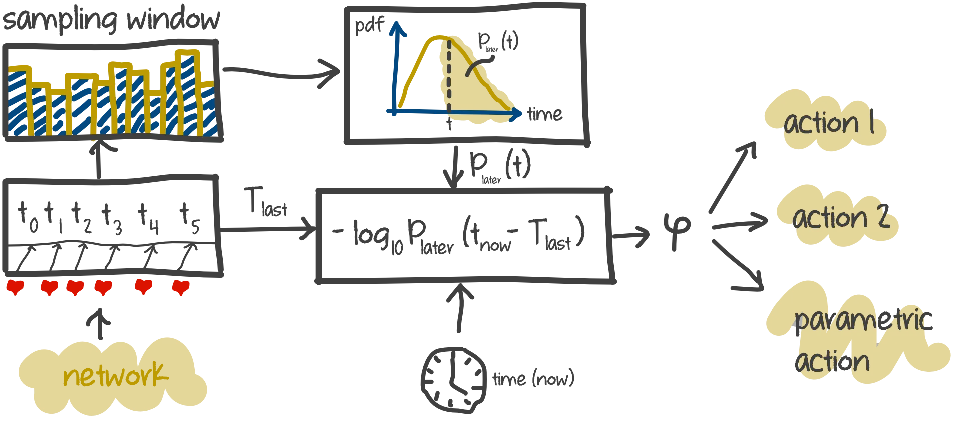
The dataflow figure above captured all the essential steps of the proposed algorithm. From the network, heartbest signal is collected and its time period is stored in the sampling window. To my understanding, the sampling window is a FIFO unit that removes oldest data when new data is added. The mean and variance for the probabilistic model $P_{later}(t)$ is then computed using the data in the sampling window. At every time step, the value of $\varphi$ is computed using the probabilistic model, the time of last arrival and the current time. This value $\varphi$ will then be used in different application for various action. For example, in action 1, the threshold for $\varphi$ is $\Phi_1$ . Let’s say in this moment, $\varphi > \Phi_1$ , hence the machine will perform action 1 (e.g. warning, reallocate resources, etc.). On the other hand, action 2 has the threshold of $\Phi_2$ , which is larger than $\varphi$ at the moment, hence no action is performed. More interestingly, the multi-level suspicion $\varphi$ enables the use of parametric action, which means the machine doesn’t have to behave in a binary manner (performs action or not), but it can perform actions to a certain degree adapting to the current situation.

Experiment

As mentioned above, the setting for experiment is a heartbeat signal transmission between Switzerland and Japan. Three failure detection schemes are compared: Chen FD, Bertier FD, and (this) $\phi$ FD. The window size of 1,000 is used for all failure detectors. In this paper, the authors conducted 4 experiments:

Exp1: Average mistake rate $\lambda_M$ . This experiment aims to provide some reasoning between the average mistake rate and the threshold $\Phi$ .
Exp2: Average detection time $T_D$ . In this experiment, the relation between average detection time and the threshold is studied. Consistent with what I mentioned above, while the average mistake rate $\lambda_M$ decreased with high threshold (8-12), the detection time is increased significantly.
Exp3: Effect of window size. The window size is plotted against the mistake rate. There are three lines representing 3 values of $\Phi$ : 1,3,5. The result showed that larger widnow size leads to lower mistake rate. The result for different values of $\Phi$ is also consistent with experiment 2.
Exp4: Comparision with Chen FD and Bertier FD. The authors conducted two experiment in this category. First experiment is comparision in the internet setting and the second is in the LAN setting. In both experiment, $\phi$ FD outperformed the other two methods.

More detail is provided in the authors’ paper.

Conclusion

This post only provides very high level abstraction of the authors’ work. I left out many discussion on the propertiesof failure detector, time period or heartbeat signal and the effect of network delay. Nevertheless, the results provided in this paper showed that the new scheme doesn’t imply additional cost in term of performance while it yields much better deteciton results under the authors’ benchmark. On another note, the authors also stated that based on their experimental result, it was sufficient to use normal distribution for the probabilistic model.