Deep compression case study - AlexNet

In this post, we study the result of Song Hans’ work on AlexNet. Since the encrypting code is not provided, we analyze the decompression code provided on the author’s github repository to have a clear understanding of the compression scheme. There are two main techniques contribute to the small size of the compressed AlexNet:

1. Values clustering - Instead of having different values for each weight matrix, each layer is limited to have only 256 distinct values (convolutional) or distinct 16 values (fully connected). These values is encoded using 8-bit integer and 4-bit integer respectively.
2. Running sum encoding for the indexing array - Each weight is stored as a sparse array (only non-zero elements are stored). To avoid large indexing values (up to several millions), the index array is stored by the difference of the non-zero index and the array index only. (This scheme enables Huffman Coding to be effective later).

Binary file layout

The provided binary file AlexNet_compressed.net is organized into a header containing the number of non-zero elements in each layers nz_num and a body containing data for each layer. Each layer has 4 main parts: codebook contains the distinct float values of the layer, bias contains the bias values (no compressing for bias), spm_stream contains the integer encoding for each non-zero elements in the weight matrix, and ind_stream contains the index for each non-zero elements.

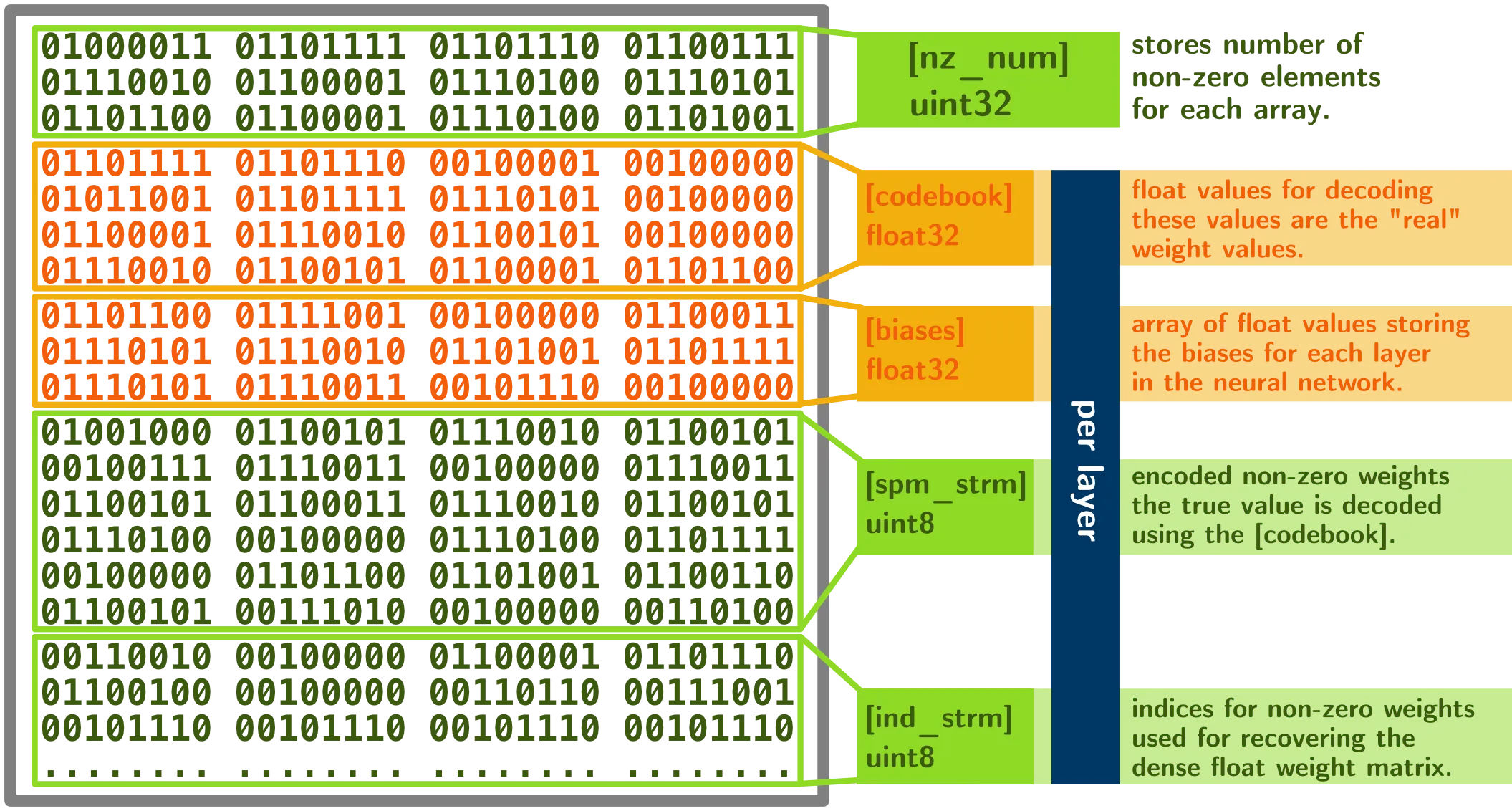
In the figure above, each part name is given corresponding to the naming in the provided decode.py file. Below the name is the size of the array (we will provide details in the following sections). Yellow stands for unsigned integer data type, blue stands for float data type.

Header

The file header contains 8 32-bit unsigned integers representing the number of non-zero elements in each layer. There are 8 layers in AlexNet. In the decompression code, this array is named nz_num.

layers = ['conv1', 'conv2', 'conv3', 'conv4', 'conv5', 'fc6', 'fc7', 'fc8']
# Get 8 uint32 values from fin (AlexNet_compressed)
nz_num = np.fromfile(fin, dtype = np.uint32, count = len(layers))
nz_num = array([29388, 118492, 309138, 247913, 163904, 4665474, 1959380, 1061645],
                dtype=uint32)

Compressed data for each layer

There are two types of layers in AlexNet namely convolutional and fully connected. As we mentioned above, each convolutional layer has 256 distinct values, while each fully connected has 16 distinct values. These distinct values are stored in codebook section as 32-bit floats. The encoding is stored as 8-bit or 4-bit unsigned integers. We take the first convolutional layer conv1 as an example.

Per layer storage layout
+----------+----------+---------------+---------------+
| codebook |  biases  |   ind_stream  |   spm_stream  |
+----------+----------+---------------+---------------+

Since conv1 is a convolutional layer, each elements in the weight matrix is encoded using 8-bit. The codebook has size 256 (of 32-bit floats):

# Read codebook from file, codebook_size=256 in this case
codebook = np.fromfile(fin, dtype = np.float32, count = codebook_size)

Bias for each convolution is read and copy to the network. In this case, there are 96 32-bit floats biases corresponding to 96 convolutional kernels. No compression was done for biases.

bias = np.fromfile(fin, dtype = np.float32, count = net.params[layer][1].data.size)
np.copyto(net.params[layer][1].data, bias)

The majority of information is stored in ind_stream and spm_stream. In the decoding process, ind_stream is read as an array of unsigned 8-bit integers. This array stores the indices of non-zero elements in the flattened weight matrix. To save storage space, ind_stream is actually stored as 4-bit integers. Thefore, each 8-bit is read as two 4-bit indices. Furthermore, the indexing is stored as the difference between a running sum of indices. The following example will make it clear:

data = [1, 3, 1, 0, 0, 0, 2, 0, 1]
ind = [0, 1, 2, 6, 8] # Only store indices of non-zero elements
ind_stream = [0, 0, 0, 3, 2] # Store the difference of a running sum
# We can get back the original index as follow:
ind = ind_stream + 1 # [1, 1, 1, 4, 2]
ind = np.cumsum(ind) # [1, 2, 3, 7, 9] - Accumulating sum
ind = ind - 1 # [0, 1, 2, 6, 8]
ind == [0, 1, 2, 6, 8] # The original indexing  

The recovering process for 4-bit indexing from 8-bit indexing is simply using bit shift:

# In here, num_nz is the number of non zero elements
ind[np.arange(0, num_nz, 2)] = ind_stream % (2**4)
ind[np.arange(1, num_nz, 2)] = ind_stream / (2**4)

The second large chunk of memory is stored at spm_stream. spm_stream stores the indexing to the codebook, which stores the real value of weights. conv1 has 256 distinct values, hence spm_stream is an array of 8-bit unsigned integers.

# Create the numpy array of size num_nz fill with zeros
spm = np.zeros(num_nz, np.uint8)
spm = spm_stream

In the case of the fully connected layer, only 16 distinct values are used. Therefore, only 4-bit is needed per element:

spm = np.zeros(num_nz, np.uint8)
spm[np.arange(0, num_nz, 2)] = spm_stream % (2**4) # last 4-bit
spm[np.arange(1, num_nz, 2)] = spm_stream / (2**4) # first 4-bit

Each element of spm_stream points to the real values in codebook. For example, if we need data[i], where i is inferred from ind_stream, we look it up at spm[i], then data[i] = codebook[spm[i]]. In here, we can clearly see that the values of fully connected layers are divided into 16 bins, and that of convolutional layers are divided into 256 bins. This is where the main compression at.

Huffman coding

Although the code provided by the author does not implement Huffman coding, we can see that Huffman coding can help to reduce the coding length for spm_stream. According to Hans, the compressed model’s size is further reduced by 1MB with the use of Huffman coding. Furthermore, it is also possible to compress the size of ind_stream due to the fact that it has multiple running streams of zeros.

Discussion

Taking a look at the weight value distribution of each layers gives some insight about the design decision for the compressed file. (For more layer encoding and clustering: weight-clustering-notebook)

The first thing we can observe here is the difference between the standard deviation of convolutional layers (conv) versus fully connected layers (fc). Moreover, the value ranges of convolutional layers are also much larger than that of fully connected layers. This observation suggests that we need to have a “finer” quantization for convolutional layers. As it turned out, to preserve the accuracy, we need to quantize the weights of a convolutional layer by 256 values; but we only need 16 discrete values for a fully connected to preserve the accuracy. This design decision is good for two reasons:

1. Larger coverage for convolutional layers. These layers are small in size (less than a million parameter each) so we can afford to encode them using 8-bits (256 values).
2. Save storage space for fully connected layers. Since a fully connected layer has up to 25 millions parameter, storing each value as a 4-bits value greatly helped to compress the size.

In a note on this compression scheme, there are several interesting points to discuss:

• Pruning parameter. We do not know the pruning threshold and the number of pruning-retraining processes. We are implementing our own pruning-clustering and codebook-training on Caffe.
• The sensitivity of quantization to the convolutional kernels. It seems that fully connected layers are more robust to quantization (limited number of distinct values than the convolutional kernels). We need to study the robustness of the pruning and quantization process with respect to the number of discrete values and the sensitivity of the values in codebook to the extracted model’s accuracy.
• The main storage lies at ind_stream (non-zero index) and spm_stream (look-up keys for real values in codebook). Can we further compress these data? One idea is to short the codebook such that the key values preserve the locality of stored values (similar keys store similar values). From here, we can store spm_stream in a lossy integer format (inspired by Fourier transformation). However, the effect of Huffman coding might be broken in this scheme.